Why Solve Mean Field Games for DeFi in the First Place?
The rise of Automated Market Makers (AMMs) such as Uniswap has triggered a wave of mathematical interest in modeling decentralized liquidity provision. At first glance, these protocols appear deterministic: trades follow a simple invariant rule, and outcomes are mechanically defined by on-chain logic. But beneath this surface lies a game.
What if the traders interacting with the pool were not passive price takers but strategic agents, each optimizing their behavior based on the actions of others? What if liquidity flow, slippage, and even gas pricing could be captured through dynamic models rooted in game theory?
That’s where Mean Field Games (MFGs) come in.
Originally developed by Lasry & Lions and Huang et al. in the late 2000s, MFGs describe strategic decision-making in large populations of agents who interact indirectly through a shared environment. Instead of modeling every trader individually, MFGs approximate the population's behavior through a representative agent responding to the "mean field" generated by the crowd. This allows tractable analysis of complex decentralized systems making it an attractive framework for DeFi.
In this project, we apply MFGs to a stylized version of Uniswap. Each agent chooses a trading intensity over time, seeking to maximize a reward function that reflects execution quality and timing. The state of the system is encoded in the liquidity pool's reserve vector, which evolves deterministically based on aggregate trading flow.
Our goal is to understand whether an individual agent, through optimal control, can meaningfully influence the pool, or whether the AMM’s design absorbs their actions like a drop in the ocean.
This blog serves as a bridge between the theoretical MFG formulation, discussed in this first post
and its numerical resolution. In doing so, we also discover an intuitive property of AMMs: their intrinsic robustness to micro-level optimization.
Numerical Methods
To solve the Mean Field Game numerically, we implemented and tested two different algorithms: a fixed-point iteration and a greedy policy iteration. Both rely on Monte Carlo simulations to approximate the law of the state trajectories under a given control or policy. Convergence is assessed based on the change in the empirical control distribution or the policy itself.
1. MFGIterativeEmpirical: Fixed-Point Iteration
This method uses a softmax-based rule to update a control distribution π_t at each time step, approximating the maximization of the intermediate reward function f. Once the distribution π_t is updated, the expected control α_t=E_π_t[a] is computed and used to generate new trajectories. The empirical distribution q_flow of controls is updated accordingly at every iteration. The algorithm continues until q_flow converges.
2. MFGPolicyIteration: Greedy Policy Iteration
In this method, we alternate between:
A policy evaluation step, where we estimate the expected reward-to-go using backward value propagation.
A policy improvement step, where we greedily choose the control that maximizes the expected return at each time step.
Unlike the fixed-point method, this iteration picks the best action rather than averaging over a distribution. However, it can be extended to use a softmax update rule as well, adding entropy regularization to smooth the control update process.
Numerical Simulation and Insights
To explore the implications of these two algorithms, we ran simulations based on the model presented in the first blog. The agents’ goal was to strategically adjust their trading rate α_t over time in order to maximize a cumulative reward f that depends on time, price trends, current state, mean field terms and the control
where
and the costs h and g are measurable in their respective domains.
We ran simulations under both methods (MFGIterativeEmpirical and MFGPolicyIteration) and analyzed how the resulting control policies affected the pool dynamics.
Evaluation Metrics
To probe the system's sensitivity to the magnitude of the reward function, we introduce a scaling factor λ:
where λ varies from 10^-4$ to 10^20. This artificial scaling allows us to see whether the numerics (and ultimately the control policy) respond to larger signals in f.
For each scaling factor $\lambda$, we track the following numerical quantities:
Max reward:
\(\max_t \max_\alpha f(t, x, \mu, q, \alpha)\)the best intermediate reward achievable.
State deviation:
\(\Delta X\)measuring how far the liquidity pool diverges from its initial value.
Max and mean control:
\(\max_t \alpha_t \text{ and } \mathbb{E}[\alpha_t] \)across time.
Control distribution change:
\(\Delta q\)indicating how far the policy deviates from uniformity.
Final cumulative reward:
\(J(\alpha)\)at convergence.
Convergence speed: Number of iterations
\(n_{\text{iter}}\)until stability.
These indicators help us assess not only how much agents influence the system, but also the efficiency and aggressiveness of their trading policy.
Simulation Parameters
All experiments are run under the same baseline settings to ensure comparability across different scales of trader impact:
Time discretization: Δt=0.01, over N=100 steps.
Action space: A=[−1,1], discretized into 11 equidistant points.
Initial state: Traders start with x_0 = 10; the liquidity pool size is X_0 = 100.
Price invariant constant: k = 1.
Intermediate cost function: h(t,x)=0.
These settings reflect a simplified but interpretable AMM environment, designed to highlight how trading behavior aggregates at scale. All solvers are implemented using Monte Carlo sampling over state trajectories and iterate until convergence in the empirical control distribution q_flow.
Interpretation of Numerical Behavior
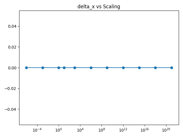
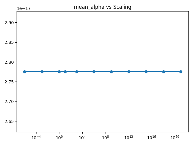
The numerical results consistently indicate that the system remains insensitive to control inputs for a wide range of reward scalings. In particular, even when the reward magnitude max f becomes significant (for instance, when λ≥10^20), the optimal control α and the state trajectory X remain virtually unchanged throughout the simulations.


Quantitatively, we observe that ΔX=0 and mean(α)=0 for all values of λ.
This outcome stems from the structure of the AMM's price impact function, where a cubic denominator in f strongly dampens the marginal effect of the agents’ actions. As a consequence, small controls (i.e., ∣α∣≪X_0) are absorbed by the system and fail to shift the state or generate noticeable rewards.
This robustness to control perturbations aligns with the analytical properties of the model and reinforces the idea that the AMM behaves stably in the presence of weak trading signals. In practical terms, unless the aggregate control across agents becomes comparable to the pool size X_0, the system dynamics remain trivial. We explicitly avoid simulating this latter case, as it would likely result in pool depletion or protocol failure, which lies beyond the scope of our current model.
Implications for DeFi and AMM Design
The numerical results presented here carry an important practical message for the DeFi ecosystem.
While it is tempting to model agents with strategic control over their trades, especially when using frameworks like Mean Field Games, the reality is that most DeFi systems are structurally robust to small agents' actions. In our model, even optimal strategies fail to shift the pool state unless the agents' aggregate action rivals the pool’s size. This reflects what we often observe in real-world AMMs: liquidity depth acts as an absorber of small noise, making individual trades largely irrelevant to price or reserve dynamics.
This has two major implications:
Modeling simplifications are justified: In many academic and industrial studies of AMMs, agents are treated as passive or price-taking. Our numerical analysis gives theoretical support to this simplification, showing that under standard liquidity assumptions, strategic behavior only matters at very high scales.
Protocol safety under mild manipulation: The cubic structure of the price impact in our model mirrors how many AMMs are designed to resist price manipulation. By penalizing large trades nonlinearly, they effectively neutralize any incentive to game the system with small or coordinated actions. This is a core principle behind mechanisms like constant product curves, slippage penalties, or even dynamic fee models.
Moreover, this experiment showcases the value of using MFGs as a simulation playground. Even when the equilibrium is trivial, the numerical framework allows us to stress-test the sensitivity of protocols to various behaviors, something especially relevant in protocol audits or economic design stages.
In future work, we aim to explore what happens when these assumptions break: What if agents have leverage? What if liquidity thins out in crises? These are the kinds of scenarios where control becomes critical and robustness must be tested.
Final Thoughts
This blog is part of a broader research effort during my PhD to understand how mathematical tools like Mean Field Games can illuminate the dynamics of DeFi protocols. Beyond the math, the goal is to build intuition and simulation frameworks that help both academics and protocol designers reason about resilience, incentives, and edge cases. Even when the answer is “nothing happens,” there’s something valuable in seeing why nothing happens and under which assumptions that might change.


